ICRA 2026

Refinery

Active Fine-tuning and Deployment-time Optimization for Contact-Rich Policies

1University of Southern California 2NVIDIA 3University of Washington 4University of Sydney
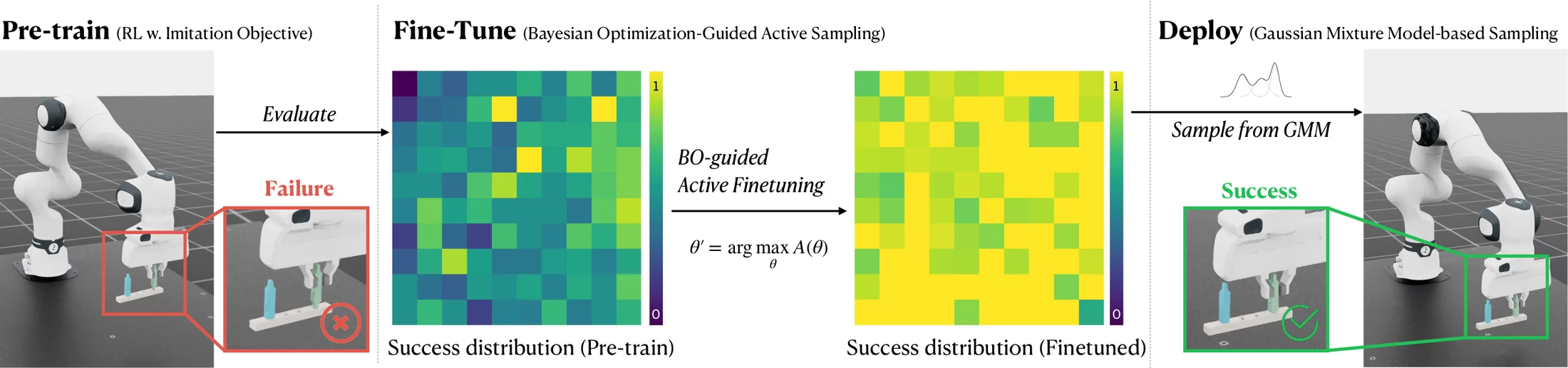
Three-stage overview. Pre-train: an RL policy trained with an imitation objective fails from some initial plug positions. Fine-tune: the policy is evaluated to build a success-rate map over initial x-y positions, which is mostly low and uneven; Bayesian-Optimization-guided active fine-tuning turns it almost uniformly high. Deploy: initial positions are sampled from a Gaussian Mixture Model fit to successful rollouts, producing a successful insertion.
Swipe the figure sideways to see detail. Method overview. We pretrain RL policies for assembly and evaluate them over initial conditions — here a success map over initial x- and y-coordinates. Bayesian Optimization-guided fine-tuning improves policy performance, and Gaussian Mixture Model-based sampling at deployment selects initializations that maximize execution success.

Video overview

Abstract

Simulation-based learning has enabled policies for precise, contact-rich tasks (e.g., robotic assembly) to reach high success rates (~80%) under high levels of observation noise and control error. Although such performance may be sufficient for research applications, it falls short of industry standards and makes policy chaining exceptionally brittle. A key limitation is the high variance in individual policy performance across diverse initial conditions.

We introduce Refinery, an effective framework that bridges this performance gap, robustifying policy performance across initial conditions. We propose Bayesian Optimization-guided fine-tuning to improve individual policies, and Gaussian Mixture Model-based sampling during deployment to select initializations that maximize execution success. Using Refinery, we improve mean success rates by 10.98% over state-of-the-art methods in simulation-based learning for robotic assembly, reaching 91.51% in simulation and comparable performance in the real world. Furthermore, we demonstrate that these fine-tuned policies can be chained to accomplish long-horizon, multi-part assembly — successfully assembling up to 8 parts without requiring explicit multi-step training.

91.51%
Mean success over 100 two-part assemblies in simulation
Baseline (AutoMate): 80.53%
+10.98 pts
96.35%
Mean per-step success across 26 multi-part assembly steps
Baseline: 83.61%
+12.74 pts
97/100
Real-world trials solved on 10 two-part assemblies
Baseline: 76/100
+21 trials
8 parts
Longest assembly chained zero-shot from per-step policies
No explicit multi-step training
Sim & real

Method

A policy with a given average success rate does not fail uniformly at random. It succeeds from certain initial states and fails from others, with high spatial variance. Refinery exploits that structure twice: it spends fine-tuning on the states the policy is most uncertain about, and at deployment it starts from the states the policy is most likely to solve.

1
Training time

Bayesian Optimization-guided fine-tuning

The success-rate landscape over initial states is unknown, non-convex, non-differentiable, and expensive to evaluate — and it moves as the policy learns. We model it with a Gaussian Process over θ, the initial xyz position of the plug relative to its goal:

Ĵi(θ) ~ 𝒢𝒫( μ(θ), k(θ, θ′) )

Each iteration re-evaluates the current policy to update the GP, then an acquisition function proposes where to fine-tune next:

θ′ = arg maxθ A(θ)

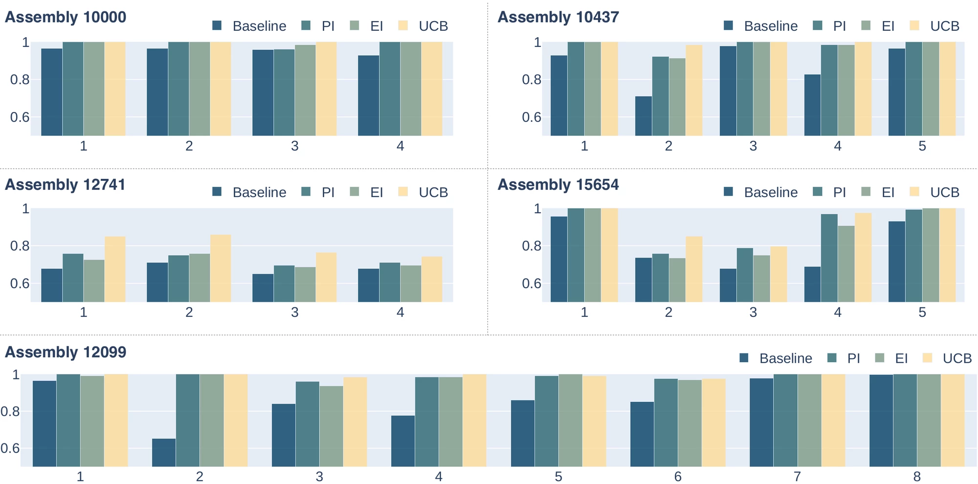
We compared three acquisition functions across all 26 steps of the 5 multi-part assemblies (5 seeds, 1000 trials each). UCB wins — exploring high-uncertainty states beats chasing the current best.

  • UCB A = μ(θ) + βσ(θ)  ·  94.41% (β = 2.0)
  • PI A = Φ( (μ(θ) − J⁺) ∕ σ(θ) )  ·  91.82%
  • EI A = (μ(θ) − J⁺)Φ(Z) + σ(θ)φ(Z)  ·  91.12%
Algorithm 1 — per assembly step
  1. Train a specialist policy πi with on-policy RL + an imitation objective (AutoMate)
  2. Evaluate the success-rate distribution Ji(θ) over plug initializations
  3. Propose samples θ′ by maximizing the acquisition function
  4. Fine-tune with episodes initialized at θ′; repeat until convergence
2
Deployment time

GMM sampling over initial conditions

Fine-tuning flattens the success landscape; deployment exploits whatever structure remains. Offline, we roll out the policy from N = 1000 uniformly-sampled initial poses, keep the successful ones, and fit a Gaussian Mixture Model to that set:

pGMM(x) = Σk ξk 𝒩( x | μk, Σk )

Online, we draw M = 1000 candidates from the mixture and start the robot at the highest-density one — no brute-force search over the initialization space:

x* = arg maxj pGMM(x̃j)

This costs nothing at training time and needs no online adaptation. On its own it lifts mean per-step success from 83.61% to 94.50%; combined with fine-tuning it reaches 96.35%. For the real robot, the GMM is fit entirely from simulation rollouts and transferred zero-shot.

Algorithm 2 — offline, then online
  1. Sample N initializations uniformly from the initialization space
  2. Execute π from each; record binary success yi
  3. Fit a GMM with K components to the successful set
  4. Sample M candidates, select the max-density one, execute
Cost. Fine-tuning converges in 50 epochs versus 200 for training from scratch, and evaluating 1000 rollouts takes seconds on a single GPU — the success-rate landscape is cheap to measure because it is measured in parallel in simulation.

Results — Simulation

Ablation across 26 multi-part assembly steps 5 seeds × 1000 trials

Each component alone adds roughly 11 points of mean success over the baseline. Fine-tuning and GMM sampling attack different parts of the problem, so stacking them lands higher than either — and halves the spread across steps, which is what makes chaining viable.

Mean per-step success rate

Averaged over 26 assembly steps from the 5 multi-part assemblies · whiskers show ±1 s.d. across steps

Baseline & single components Refinery (both) ±1 s.d. across steps

Baseline = train from scratch, uniform initialization · + GMM deploy = baseline policy, GMM-sampled initialization · + BO fine-tune = UCB-fine-tuned policy, uniform initialization · Refinery = both.

Mean per-step success rate across 26 multi-part assembly steps
ApproachMean success rate (%)Standard deviation
Baseline (AutoMate)83.619.27
GMM deployment-time sampling only94.504.90
Bayesian Optimization fine-tuning only94.417.51
Refinery (both)96.354.45

100 two-part assemblies Does fine-tuning beat the state of the art?

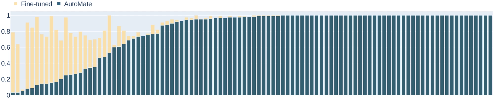
Fine-tuning the AutoMate specialist policies with UCB raises mean success from 80.53 ± 31.43% to 91.51 ± 14.27% — a 10.98-point gain in the mean and a 17.16% reduction in variance. The gains concentrate exactly where they are needed: the policies that were nearly hopeless.

Stacked bar chart of 100 two-part assembly tasks sorted by baseline success rate. Dark teal bars show AutoMate baseline success; pale sand bars stacked on top show the additional success gained by fine-tuning. The leftmost third of tasks, where the baseline is near zero to 0.5, gains the most, with many fine-tuned policies reaching close to 1.0. Tasks already near 1.0 stay there.
Swipe the figure sideways to see detail. Per-task success on the 100-assembly benchmark. Policies are sorted by baseline success rate. The sand segment is the improvement contributed by BO-guided fine-tuning; the hardest tasks improve the most, and many fine-tuned policies approach or reach 100%.

Which acquisition function? UCB, PI, or EI

Per-step success for every acquisition function on all 5 multi-part assemblies. UCB (94.41%) leads PI (91.82%) and EI (91.12%), all well clear of the 83.61% baseline. The advantage is largest on the hardest assembly, 12741, where exploration of uncertain initial states matters most.

Five grouped bar charts, one per multi-part assembly (10000, 10437, 12741, 15654, 12099). Within each, every assembly step shows four bars: Baseline, PI, EI and UCB. The UCB bar is highest or tied in most steps, and the gap over baseline is widest for assembly 12741 where baseline steps sit near 0.65 to 0.71 and UCB reaches 0.74 to 0.86.
Swipe the figure sideways to see detail. Acquisition-function comparison. Success rate per assembly step for each acquisition function across the 5 multi-part assemblies. The x-axis is the step index within each assembly.

Fine-tuning vs. deployment sampling, step by step

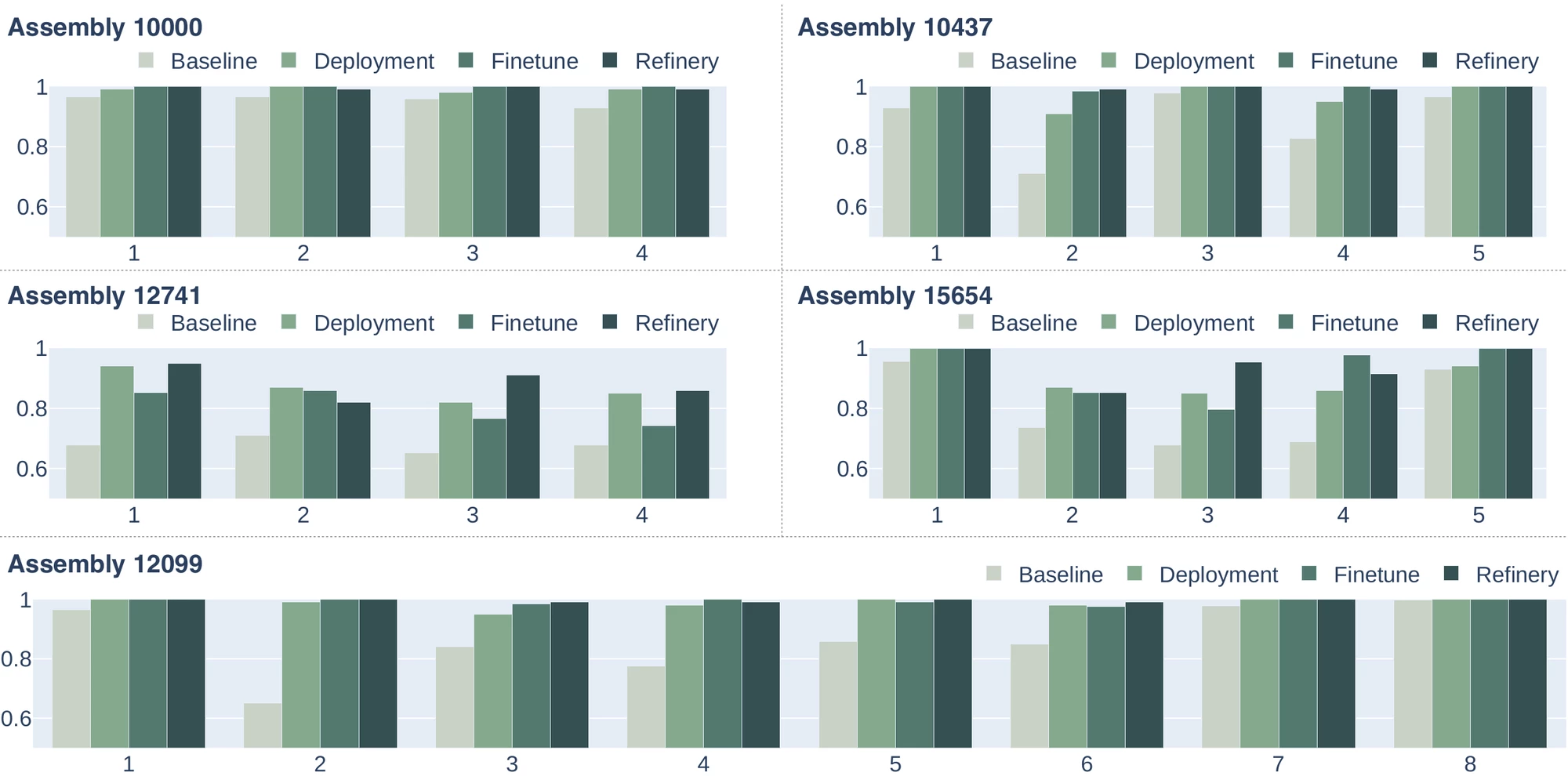
The same ablation as the chart above, resolved per assembly step. GMM sampling alone already recovers most of the gap without touching the policy — but the combination is the most consistent, and is the only configuration that stays high on the difficult assemblies 12741 and 15654.

Five grouped bar charts, one per multi-part assembly. Within each, every step shows four bars: Baseline, Deployment, Finetune and Refinery, in a pale-to-dark sage ramp. Refinery is highest or tied in most steps. On assemblies 12741 and 15654 the baseline bars drop to around 0.65 to 0.74 while Refinery stays between 0.82 and 1.0.
Swipe the figure sideways to see detail. Per-step ablation. Success rate under each combination of fine-tuning and deployment-time sampling strategy, across the 5 multi-part assemblies.

Full assembly sequences All steps must succeed

Sequence-level success, where a trial counts only if every step succeeds. This is where per-step variance compounds — and where Refinery's gains are largest. Assembly 12099 (8 steps) goes from a 31.26% sequence success rate to 97.68%.

Full assembly sequence success rates (%) for five multi-part assemblies under four approaches
Assembly Steps Baseline Deployment Fine-tune Refinery (ours)
10000483.2096.47+13.2799.22+16.0298.45+15.25
12099831.2691.55+60.2991.52+60.2697.68+66.42
12741421.1056.78+35.6848.65+27.5560.62+39.52
10437549.1186.45+37.3498.44+49.3398.44+49.33
15654531.9856.48+24.5066.22+34.2474.19+42.21

Success rates in %. Deployment = GMM sampling only · Fine-tune = BO fine-tuning only · Refinery = both. Bold marks the best result per assembly.

Results — Real World

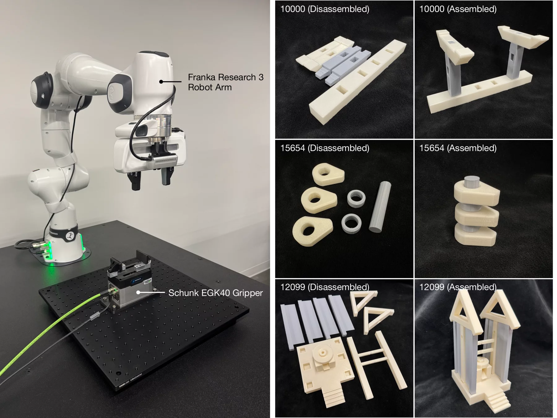
A Franka Research 3 arm with a parallel-jaw gripper, a table-mounted Schunk EGK40 gripper acting as a fixture, and 3D-printed parts from our dataset. Policies and the deployment-time GMM are trained entirely in simulation and transferred without real-world adaptation.

Left: a Franka Research 3 robot arm with a parallel-jaw gripper above an optical breadboard holding a Schunk EGK40 gripper used as a fixture. Right: six photographs of 3D-printed assemblies 10000, 15654 and 12099, each shown disassembled as loose cream and grey parts and assembled into its final structure.
Real-world setup. Franka Research 3 robot and a table-mounted Schunk EGK40 gripper perform multi-part assembly. 3D-printed assemblies 10000, 15654 and 12099 are shown disassembled and assembled.

10 two-part assemblies 300 real trials

Ten trials per assembly per approach. Refinery solves 97/100 trials against the baseline's 76/100. On the three hardest assemblies (01053, 00190, 00514) real-world success goes from 12/30 to 27/30; on the four mid-range ones it eliminates every residual failure, 3/40 down to 0/40.

Simulation success rate and real-world trials solved for ten two-part assemblies under three approaches
Assembly Baseline Fine-tune Refinery (ours)
Sim %Real Sim %Real Sim %Real
0105356.252/1091.417/1097.669/10
0019054.694/1087.3410/1099.2210/10
0051476.566/1088.288/1089.848/10
0061484.378/1089.699/1091.8610/10
0068194.538/1096.878/10100.0010/10
0055392.189/1094.5310/1097.6610/10
0076896.879/1098.4410/1099.2210/10
0034697.6610/10100.0010/10100.0010/10
01036100.0010/10100.0010/10100.0010/10
0112996.8810/10100.0010/10100.0010/10
Total 84.9976/100 94.66+9.6792/100+16 97.54+12.5597/100+21

Only Refinery uses GMM-based initialization at deployment, and the GMM is fit directly from simulation data.

Multi-part sequences on the real robot 160 subtask executions

Three multi-part assemblies, 10 full-sequence trials each. Per-step reliability is strong — 146/160 = 90.6% fully autonomous — but whole sequences remain the hard case, since one bad step ends the trial. The gap between the "fully autonomous" and "1 intervention" columns shows how much of the remaining loss comes from a single failing step.

Real-world multi-part assembly: per-step success and full-sequence success with zero, one or two human interventions
Assembly Individual steps Fully autonomous ≤ 1 intervention ≤ 2 interventions
1000037/408/1010/1010/10
1209965/706/1010/1010/10
1565444/505/109/1010/10
Total146/16090.6%19/3029/3030/30

To our knowledge this is the first demonstration of zero-shot sim-to-real for multiple long-horizon, multi-part assemblies.

Dataset

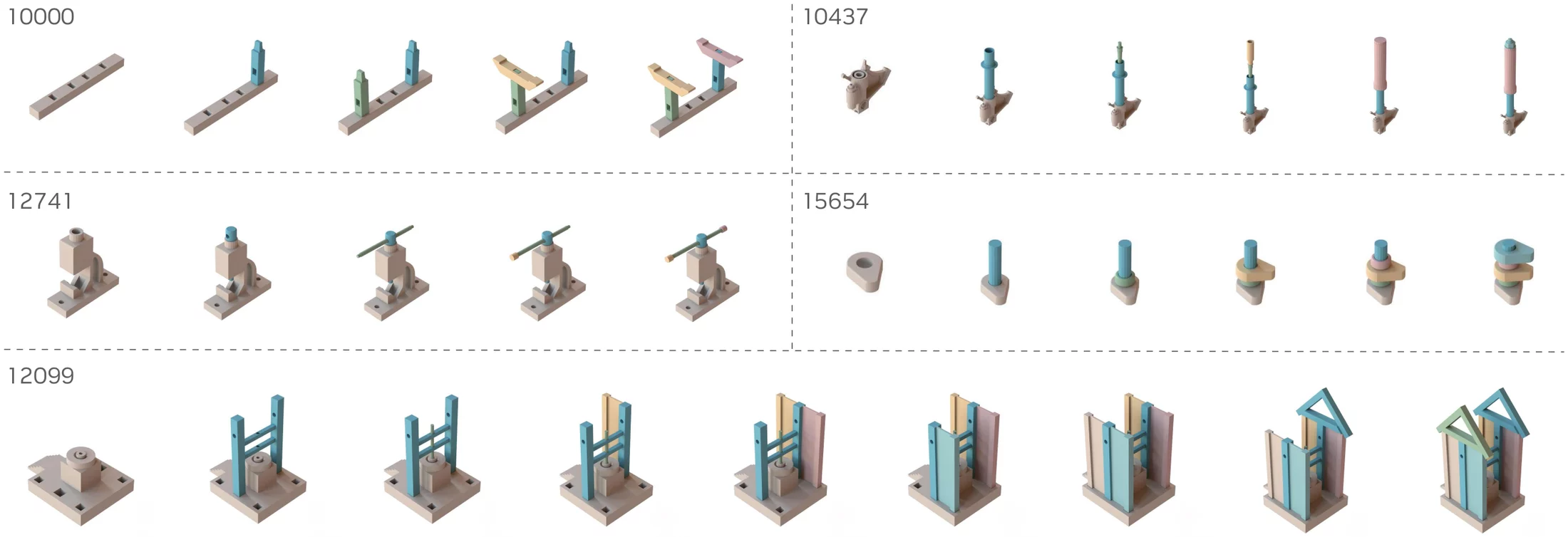
We contribute a geometrically-diverse dataset of multi-part assemblies derived from ASAP, together with the corresponding simulation environments. Each assembly has 5–9 components and 4–8 discrete insertion steps, every component is graspable by a parallel-jaw gripper, and the whole sequence is executable by a single arm with each part added atop the parts already placed in a static fixture.

Rendered assembly sequences for five assemblies labelled 10000, 10437, 12741, 15654 and 12099. Each row shows the structure growing one pastel-coloured part at a time, from a single base component on the left to the complete assembly on the right. Assembly 12099 is the longest with nine frames.
Swipe the figure sideways to see detail. Multi-part assembly dataset. Assembly sequences for the 5 multi-part assemblies, derived from ASAP. Each frame adds one part to the partially-assembled structure.
Preparation. Component meshes are scaled into a 10 cm³ bounding box, reoriented so the base stands upright on the z-axis, translated so the base's bottom face is coplanar with the origin, and depenetrated to enforce 0.5 mm clearance between parts — leaving the dataset compatible with non-penetration simulators and directly 3D-printable.

Limitations

We traced the residual failure cases in both simulation and the real world to three causes.

  • Grasp instabilityThe parallel-jaw gripper slips or introduces unintended rotations while transporting a part — robustness in grasping, not insertion, is the bottleneck.
  • Disturbing prior partsDuring multi-step assembly the robot can apply large forces that destabilize or displace already-assembled parts. Integrating force control is a natural next step.
  • 3D-printing tolerancesReal parts flex or mismatch the source mesh because of printer settings — a failure mode no policy can correct for.

BibTeX

@inproceedings{tang2026refinery,
  title     = {Refinery: Active Fine-tuning and Deployment-time Optimization
               for Contact-Rich Policies},
  author    = {Tang, Bingjie and Akinola, Iretiayo and Xu, Jie and Wen, Bowen
               and Fox, Dieter and Sukhatme, Gaurav S. and Ramos, Fabio
               and Gupta, Abhishek and Narang, Yashraj},
  booktitle = {IEEE International Conference on Robotics and Automation (ICRA)},
  year      = {2026}
}